Modeling Capabilities

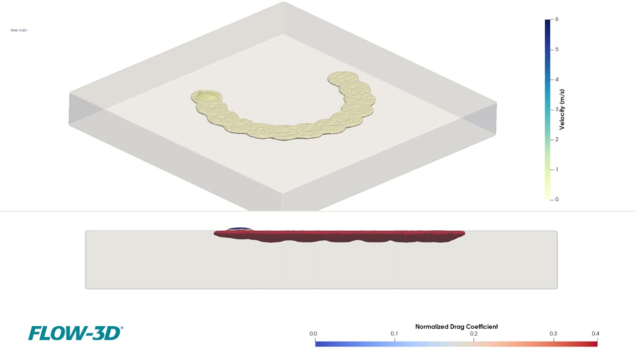
The new droplet/bubble source model allows either spherical droplets or bubbles to be emitted at defined intervals from a point source. This source can be either stationary or its motion can be defined in a tabular fashion. The initial velocity of the droplet or bubble can also be defined in three dimensions. All physical models are compatible with this model so that typical applications such as porous media flow, evaporation/solidification, and surface tension can be simulated. In this example, a droplet source moves in a circular pattern while ejecting droplets downward at a velocity of 10 m/s into a porous medium to create a ring-shaped design.

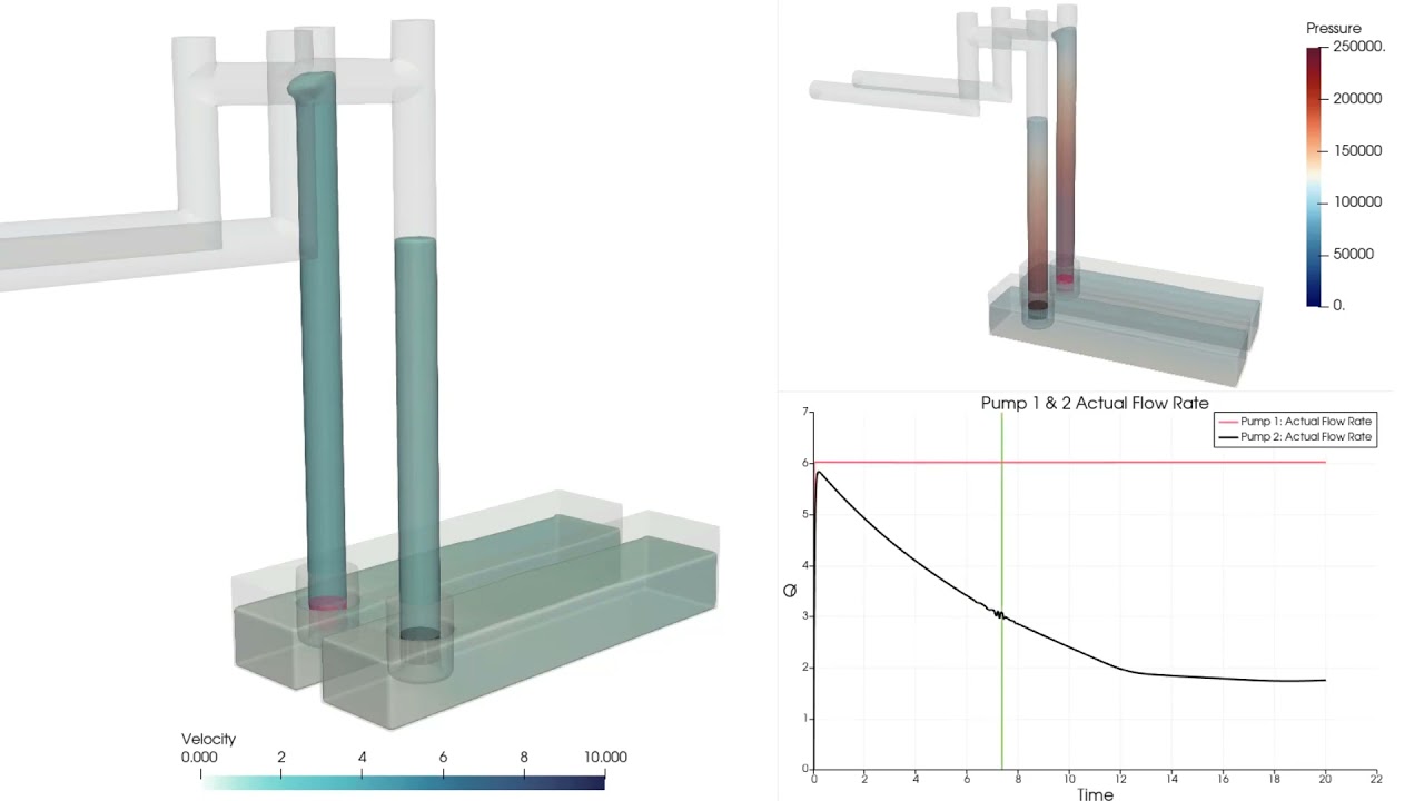
FLOW-3D’s new axial pump model allows users to mimic the net effect of an axial pump in their simulations. There are two options with respect to the pump behavior. The first option is to prescribe either a volumetric flow rate or a flow velocity through the pump so that the fluid is moved at the specified rate. This option is appropriate when an operating flow rate is provided for the pump. The second option provides a more complete definition of the pump operation based on a pump performance curve.

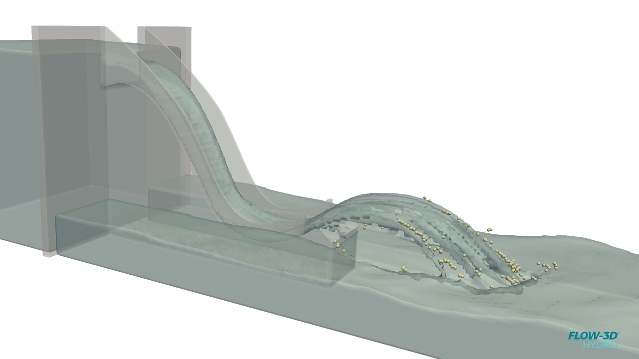
The accuracy and robustness of the sharp-interface tracking VOF methods in FLOW-3D have been enhanced by combining them with fluid particles. The new particle species, called VOF particles, are used in place of the VOF function to track small fluid ligaments and droplets in the computational domain, achieving better conservation of fluid volume and momentum.

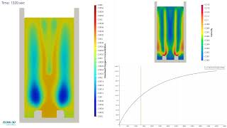
In this simulation, oxygen bubbles are injected from two diffusers at the bottom of the container and allowed to rise in water. As the bubbles rise, oxygen dissolves into water. The image on the left shows the concentration of dissolved oxygen in water. The image on the right shows the water velocity which is induced by the rising oxygen bubbles.

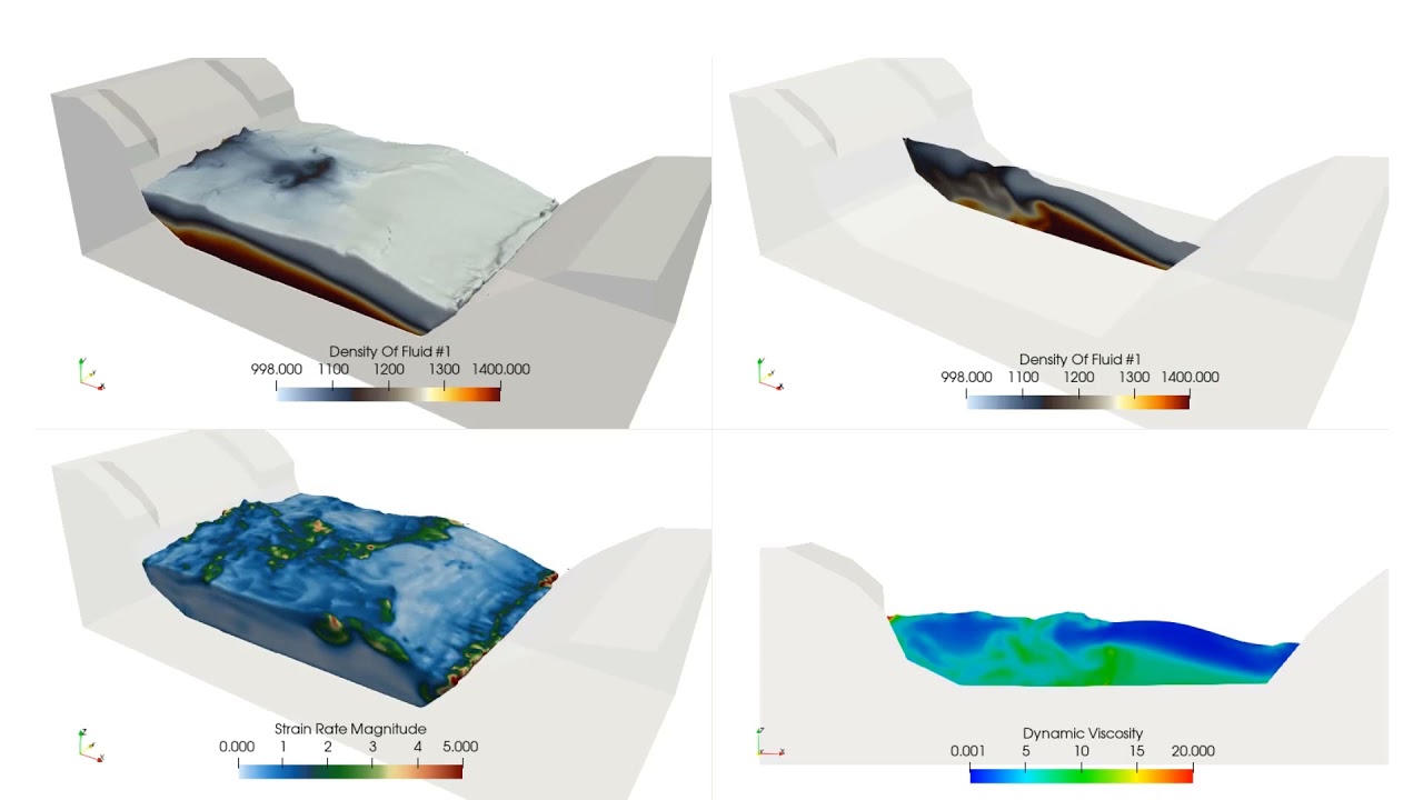
Viscosity is defined as a function of both solid content (density) and strain rate. In this example a dense fluid region slides down into a quiescent pool which at time zero is layered with a dense settled fluid region and clear water above.

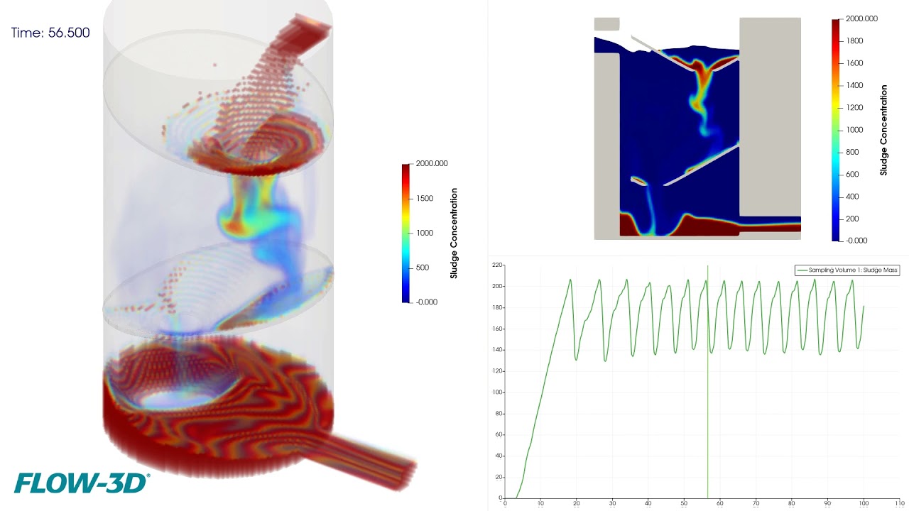
This example represents a sludge decanter that models a mixture of water and sludge entering a decanter and separating. Water is allowed to flow in and out at the back side of the decanter to maintain a relatively fixed level in the decanter. A sampling volume in the bottom of the decanter is used to measure the amount of sludge captured at the bottom. When the sludge mass in the sampling volume reaches 200 kg, a valve opens to release the sludge. The valve closes when the sludge mass drops below 180 kg.

This example demonstrates FLOW-3D‘s capabilities for simulating a material extrusion AM process. In this simulation, a single strand of highly viscous material is extruded and deposited on a stationary substrate. The heat transfer model is activated, and the density is evaluated as a function of strand temperature after the deposition, which allows the material shrinkage to be predicted. The example is post-processed with FLOW-3D POST.

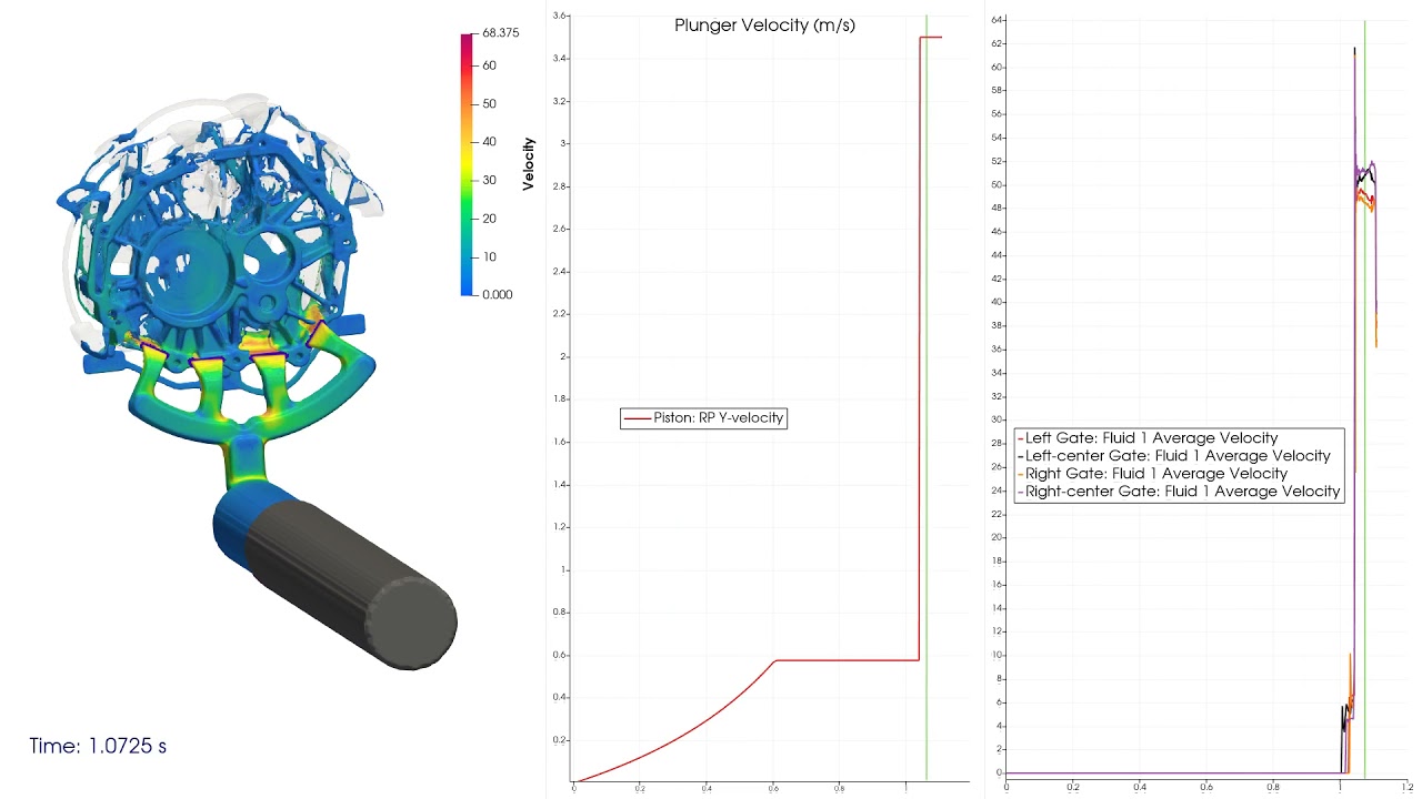
This video demonstrates Active Simulation Control being used to increase data output frequency when fast shot begins so that flow details can be captured. Flux surfaces are placed at the gates to measure the average velocity. When the average velocity exceeds 35 m/s, Active Simulation Control sets the output frequency to 0.0007 seconds for the duration of the simulation.

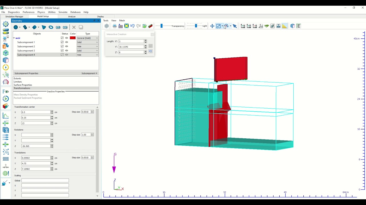
FLOW-3D‘s interactive geometry creation and editing is better than ever, and now includes new interactive tool selection including rotate, move and resize; enter rotate, move, or resize mode by clicking the action and selecting the geometry to modify; and clicking the up arrow icon or hitting the ESC key will return the user to a normal select mode.

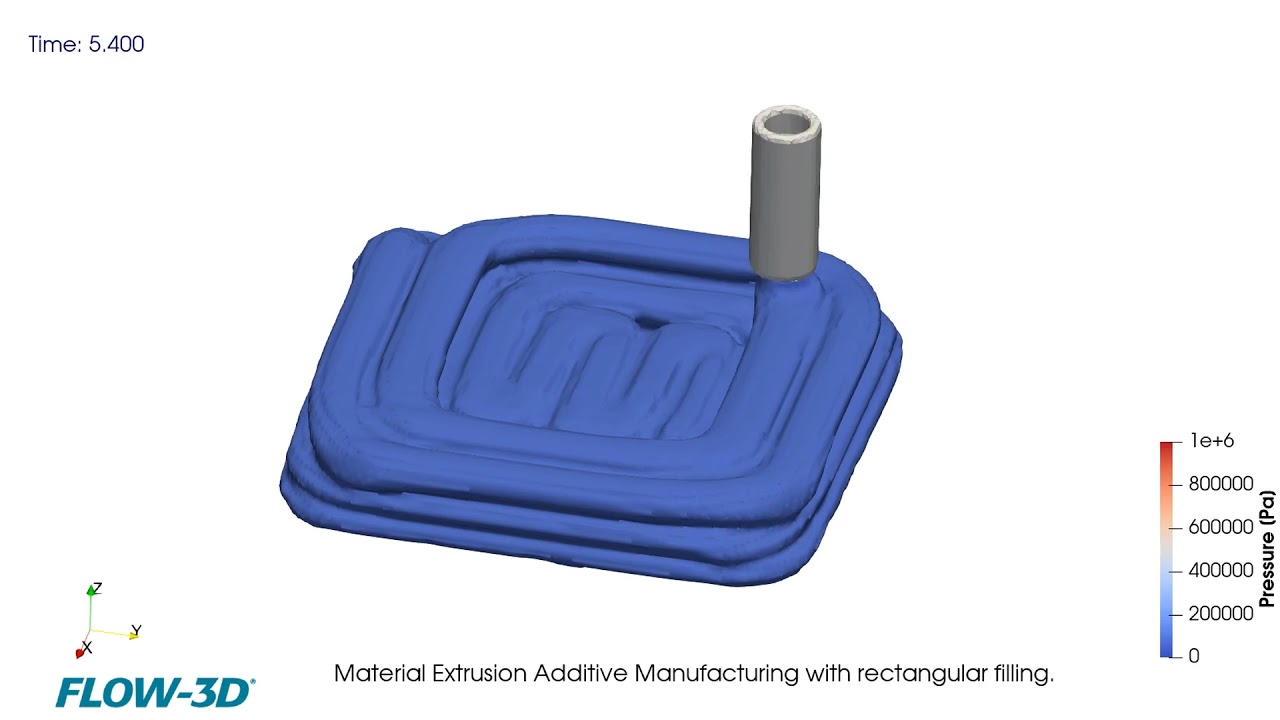
This example demonstrates FLOW-3D‘s capabilities to simulate a material extrusion AM process. In this simulation, the material is approximated as a highly viscous fluid with constant material properties. Four layers with rectangular filling are printed and the deformations of already deposited material under the newly extruded strands can be observed. The example is post-processed with FLOW-3D POST.

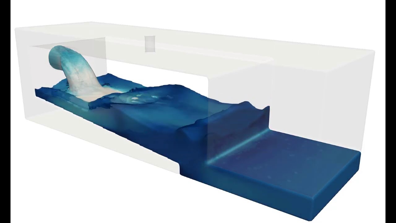
This pre-packaged FLOW-3D HYDRO example of a discharge into a tank uses the Free surface – 2 fluid VOF template available in FLOW-3D HYDRO for users to quickly setup two phase air/water models. Air and water properties, and all the appropriate models and numerical settings are pre-loaded into the simulation, providing a great starting point to model two phase flows, from setup through to post-processing analysis. Learn more about FLOW-3D HYDRO‘s complete CFD solution for the civil and environmental engineering industry at https://www.flow3d.com/products/flow-3d-hydro/water-treatment/

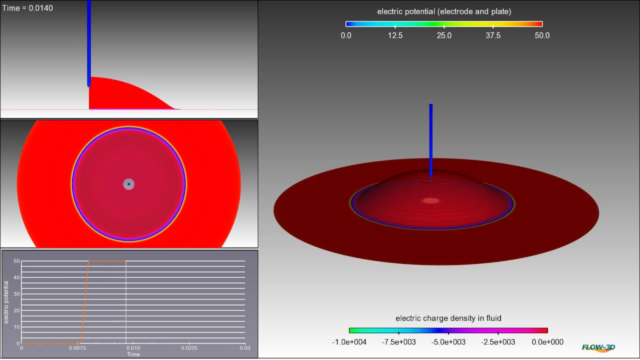
Electrowetting is a technique used to change the apparent contact angle of a dielectric fluid under the influence of electric potential. In this example, the fluid is originally hydrophobic and beads on the surface. However, when a 50V potential difference is applied, the fluid is forced to wet the surface becoming hydrophilic.

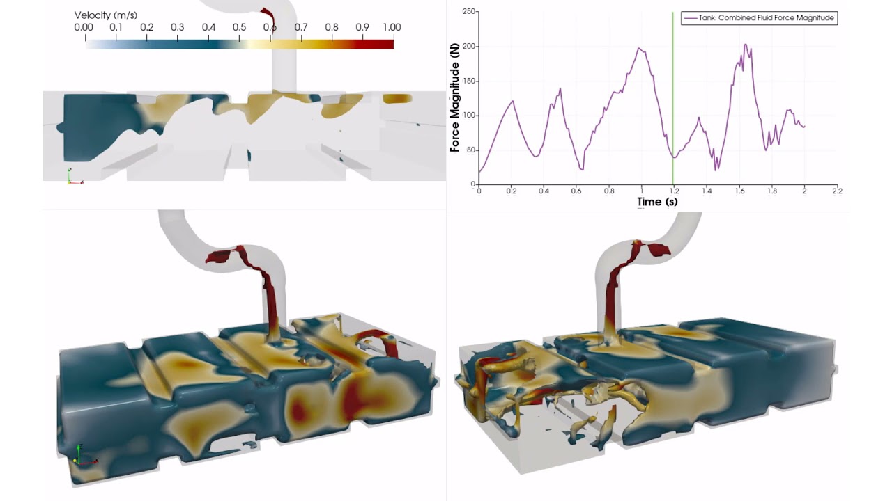
Automotive fuel tanks hold significant fuel mass and are subject to constant vehicle accelerations and decelerations. This presents a structural issue for tank material due to the impact forces. Additionally, sloshing of fuel can cause incorrect reading or damage to measurement devices. Shown here is a simulation in FLOW-3D of fuel sloshing under acceleration plotting velocity contours. The graph shows transient force magnitude on fuel tank. Learn more at https://www.flow3d.com/industries/automotive/

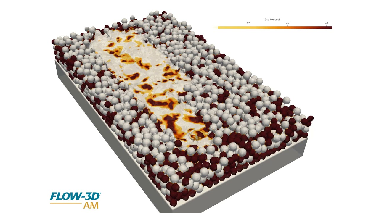
Micro and meso scale simulations using FLOW-3D AM help us understand the mixing of different materials in the melt pool and the formation of potential defects such as lack of fusion and porosity. In this simulation, the stainless steel and aluminum powders have independently-defined temperature dependent material properties that FLOW-3D AM tracks to accurately capture the melt pool dynamics. Learn more about FLOW-3D AM‘s mutiphysics simulation capabilities at https://www.flow3d.com/products/flow3d-am/

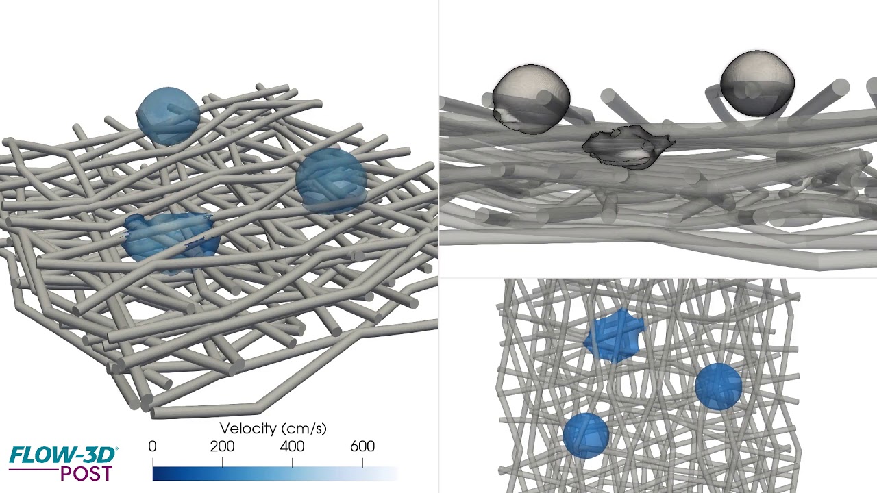
Here, FLOW-3D is used to simulate drop impingement on a fibrous bed, looking at the propagation of the fluid front as it relates to surface tension, contact angle, and viscosity. For more information on this and other coating simulation capabilities, visit https://www.flow3d.com/industries/coating/