

Solving the World’s Toughest CFD Problems
Salt dissolution in liquid is involved in many CFD applications—from solution mining to food processing to medical applications. The Salt Dissolution model in FLOW-3D accounts for basic physical phenomena, such as mass transfer at the interface between salt and fluid, the change of volume and shape of the solid salt, diffusion and convection of dissolved salt in fluid and, finally, the change in fluid density, viscosity and surface tension.
The amount of dissolved salt in liquid is represented with its mass concentration C. The mass flux of salt, Q, at the liquid/solid salt boundary is defined as Q = k (CSAT – C), where k is the constant mass transfer coefficient and CSAT is the saturation concentration of salt. The fluid mixture density is assumed to be a linear function of the salt concentration. The fluid volume can also vary with concentration. For example, the density of the saturated sea water (brine) at room temperature is about 26% greater than the density of fresh water, while its volume increases by 13%.
Once the dissolved salt has been apportioned to the computational domain, diffusion and convection take over and further redistribute the salt within the mixture. The model accounts for the presence of solid salt in the flow domain, and its change in volume and shape as it is dissolved in fluid. The geometry component representing the solid salt is designated as a component of a special type: instead of moving, it changes shape and volume. The area and volume fractions are recomputed at every time step to reflect the gradual dissolution of the solid salt.
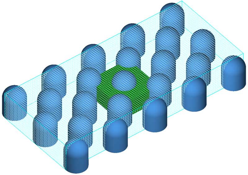
The model is illustrated using a test that approximates the dissolution of solid crystals of medicine by sweat in a skin patch. The three-dimensional geometry of the domain is shown in Fig. 1. The size of the domain is 4.5 mm by 2 mm by 0.8 mm. A regular pattern of identical cylindrical obstacles (“pins”) is defined, each pin is 0.5 mm in diameter and 0.65 mm in height.
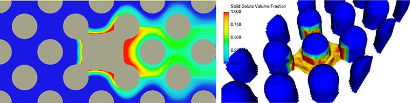
Since the salt dissolution rate is much smaller than the rate at which the domain is initially filled by fluid due to capillary forces, the problem is modeled as confined flow with a fixed flow rate along the direction shown by the arrow in Fig. 1. The results are shown in Fig. 2.
The pressure difference of 5,000 dynes yields an average flow velocity of 0.25 cm/sec. The average velocity, together with the flow rate, gradually increases as the salt dissolves since it creates more opening for the flow. The upwind side of the solid salt block dissolves faster than the downstream side because the dissolved salt is washed away by the flow. The mixture at the downstream end is more saturated and slows down the dissolution process in this area. Another observation from this particular test is that the diffusion of salt in the fluid is small compared with convection.
The salt dissolution model can be employed in a variety of situations, from salt mining to the creation of underground cavities for natural gas storage, to drug delivery, to metal alloying and more.
| Cookie | Duration | Description |
|---|---|---|
| cookielawinfo-checkbox-analytics | 11 months | This cookie is set by GDPR Cookie Consent plugin. The cookie is used to store the user consent for the cookies in the category "Analytics". |
| cookielawinfo-checkbox-functional | 11 months | The cookie is set by GDPR cookie consent to record the user consent for the cookies in the category "Functional". |
| cookielawinfo-checkbox-necessary | 11 months | This cookie is set by GDPR Cookie Consent plugin. The cookies is used to store the user consent for the cookies in the category "Necessary". |
| cookielawinfo-checkbox-others | 11 months | This cookie is set by GDPR Cookie Consent plugin. The cookie is used to store the user consent for the cookies in the category "Other. |
| cookielawinfo-checkbox-performance | 11 months | This cookie is set by GDPR Cookie Consent plugin. The cookie is used to store the user consent for the cookies in the category "Performance". |
| viewed_cookie_policy | 11 months | The cookie is set by the GDPR Cookie Consent plugin and is used to store whether or not user has consented to the use of cookies. It does not store any personal data. |
