

Detailed Cutcell Representation
The fractional cell area and volume method, FAVOR™, enables FLOW-3D to efficiently simulate flow through and around user-defined geometry, without needing unstructured, body-fitted grids. It does this by formulating the governing equations in terms of local porosity functions, which correspond to the open volume and area fractions of the grid cells. In cutcells, where geometry intersects the grid, the porosity functions are used to approximate the surface location, surface orientation, and surface area. In certain situations, these approximations can limit the accuracy of viscous boundary layers, especially along solid surfaces that cannot be aligned with mesh planes. Wall shear stress is especially sensitive to the surface treatment, and skin friction distributions generated with cutcell methods can be noisy.
The core issue at hand can be resolved by embedding a more detailed representation of the cutcell geometry in the solution (Kirkpatrick, Armfield, & Kent, 2003) (Berger & Aftosmis, 2012). The precise geometry defining each cutcell is determined from a sequence of cell-plane intersections during the preprocessing step and replaces the standard approximations made in the discrete equations. This fundamentally improves the accuracy of momentum fluxes along solid boundaries, reducing noise and improving solution quality. A new solver option now enables this detailed cutcell representation in FLOW-3D, as an additional layer on top of the standard FAVOR™ area and volume fractions. Importantly, the governing partial differential equations being solved remain the same, and the overall robustness of the solver is unchanged.
As of the 2022R1 release, the detailed cutcell representation is restricted to Cartesian mesh blocks and non-moving, non-porous components. It is also not currently compatible with the immersed boundary method (IBM) (Liang, 2018). For the time being, it is recommended to use detailed cutcells when viscous boundary layer effects are important and IBM in advection dominated situations.
Results
Several tests have been performed to benchmark the accuracy of the detailed cutcell representation in FLOW-3D 2022R1.
Laminar flow past a circular cylinder at Re=40
Incompressible flow around a circular cylinder at Reynolds number, $latex \displaystyle Re=\frac{\rho {{U}_{0}}d}{\mu }=40$ is a standard test of boundary layer accuracy (Gautier, Biau, & Lamballais, 2013). Here U0 is the free stream velocity, d is the cylinder diameter, ρ is the fluid density and μ is the fluid viscosity. The flow was simulated using three different grids with spacing, $latex \displaystyle \frac{d}{{{\Delta }_{1}}}=40,\frac{d}{{{\Delta }_{2}}}=20,\frac{d}{{{\Delta }_{3}}}=10$


Figure 1: Laminar flow past a cylinder at Re=40.
The steady state drag coefficient was calculated from the results as, $latex \displaystyle {{C}_{D}}=\frac{{{F}_{D}}}{\frac{1}{2}\rho U_{0}^{2}{d}’}$, where FD is the total drag force (pressure plus shear). Results on the three grids show convergence under grid refinement to the center of the range reported by (Gautier, Biau, & Lamballais, 2013) and agree well with other Cartesian grid solutions, including the IBM results from (Tseng & Ferziger, 2003). The pressure coefficient, $latex \displaystyle {{C}_{p}}\left( \theta \right)=\frac{p\left( \theta \right)-{{p}_{0}}}{\frac{1}{2}\rho U_{0}^{2}}$, and skin friction coefficient, $latex \displaystyle {{C}_{f}}(\theta )=\frac{\left| \tau \left( \theta \right) \right|}{\frac{1}{2}\rho U_{0}^{2}}$, were also calculated for each simulation and plotted as a function of angle from the stagnation point, θ. In these results τ is the wall shear stress, p is the surface pressure, and p0 is the far-field pressure. Agreement with experimental pressure measurements (Grove, Shair, & Petersen, 1964) and shear stress calculations from a body-fitted solver (Tseng & Ferziger, 2003) is very good.
Turbulent flow around a NACA0012 airfoil
Flow around a NACA0012 airfoil was simulated at $latex \displaystyle Re=\frac{\rho {{U}_{0}}c}{\mu }=2.88\times {{10}^{6}}$, where c is the airfoil chord length. The foil is located at the center of a 60c×60c computational domain, with an upstream velocity inlet, downstream pressure outlet, and a 10° angle of attack. Flow near the surface of the foil is discretized using a grid size, $latex \displaystyle \frac{c}{\Delta }=128$. Grid spacing is made progressively coarser away from the foil, by employing a total of 5 nested mesh blocks, each with double/half the spacing of the parent/child mesh. The RNG turbulence model was enabled with dynamic length scale calculation.
This is the same Re and foil orientation as the fully turbulent experiments of (Gregory & O’Reilly, 1970), where turbulence was tripped at the leading edge (no laminar transition). Surface profiles of the steady state pressure coefficient are compared with both experimental data (Gregory & O’Reilly, 1970) and numerical results from the body-fitted SU2 solver (Economon, Palacios, Copeland, Lukaczyk, & Alonso, 2016) in Figure 2b. Note that the SU2 results are at a somewhat higher Reynolds number of Re=6×10⁶. The FLOW-3D results for surface pressure coefficient agree very well with both datasets.
Further comparison of the skin friction coefficient on the upper foil surface with the SU2 solver is made in Figure 2c. Agreement is good, and the mismatch in peak shear stress between the two results is likely due to the different Reynolds numbers and also the coarse grid in the FLOW-3D model, which was not refined to capture the thin boundary layer at the airfoil’s leading edge.
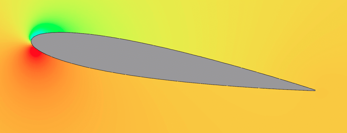


Figure 2: Turbulent flow around a NACA0012 airfoil at 10° angle of attack
Smooth and rough wall pipe flow
Steady, incompressible flow through a circular pipe with diameter, d, and surface roughness, ε, was simulated. In this case, the dimensionless shear stress or friction factor, $latex \displaystyle f\left( Re,\frac{\varepsilon }{d} \right)=\frac{8\tau }{\rho U_{0}^{2}}$, relates the shear stress to Reynolds number, $latex \displaystyle Re=\frac{\rho {{U}_{0}}d}{\mu }$ and relative roughness, $latex \displaystyle \frac{\varepsilon }{d}$. Here U0 is the mean velocity in the pipe.
For laminar flow (Re≤2100) the friction factor in smooth pipes is,
$latex \displaystyle f\left( Re \right)=\frac{64}{Re}$.
(1)
For turbulent flow through rough pipes, the Swamee-Jain (Swamee & Jain, 1976) equation provides an explicit approximation to the implicit Colebrook equation,
$latex \displaystyle f\left( Re,\frac{\varepsilon }{d} \right)=\frac{0.25}{{{\left( {{\log }_{10}}\left( \frac{\varepsilon /d}{3.7}+\frac{5.74}{R{{e}^{0.9}}} \right) \right)}^{2}}}$.
(2)
It is valid for 5000 ≤ Re ≤ 108 and 10-6 ≤ $latex \displaystyle \frac{\varepsilon }{d}$ ≤ 0.05.
The setup of this problem in FLOW-3D is shown in Figure 3. Flow travels through the pipe in the x-direction, driven by the gravitational body force, g. Periodic boundaries are used in the flow direction to eliminate pipe entrance effects. The mesh is uniform in the yz plane with $latex \displaystyle \frac{d}{\Delta }=20$ and a total of 3 cells are used in the periodic x direction (the solution is not sensitive to the number of cells in x). Three laminar Reynolds numbers, ReLaminar = [500, 1000, 2000] and six turbulent Reynolds numbers, ReTurbulent = [10000, 40000, 160000, 640000, 2560000, 10240000] were targeted by applying an appropriate body force. For each turbulent Reynolds number, a separate simulation was set up for five values of relative roughness, $latex \displaystyle \frac{\varepsilon }{d}=$[0, 0.0001, 0.001, 0.01, 0.05]. All turbulent flow simulations used the RNG turbulence model with dynamic length scale calculation. The steady state shear stress and mean velocity were used to compute the actual Reynolds number and actual friction factor from each result.


Figure 3: Illustration of the periodic pipe flow simulations. (a) shows the simulation setup in FLOW-3D . (b) shows contours of velocity magnitude at steady state for Re=10M, and the mesh resolution in the pipe cross section $latex \displaystyle \frac{d}{\Delta }=20$


Figure 4: Pipe flow simulation results. (a) shows friction factor as a function of Reynolds number for pipes having different roughness, $latex \displaystyle \frac{\varepsilon }{d}$. The solid lines are the semi-empirical equations 1 and 2. Each symbol corresponds to a single FLOW-3D simulation. (b) Circumferential variation of shear stress, τ, for the case Re=160,000, $latex \displaystyle \frac{\varepsilon }{d}$= 0.001
Friction factor is plotted as a function of Reynolds number in Figure 4a alongside the analytic/empirical curves (Equations 1 and 2) for each value of relative roughness, $latex \displaystyle \frac{\varepsilon }{d}$. Agreement with the laminar correlation is excellent and nearly all turbulent results are within the ≈10% uncertainty range associated with Equation 2. Figure 4b shows the circumferential variation of the shear stress for all points on the surface of the pipe for the case Re=160,000, $latex \displaystyle \frac{\varepsilon }{d}$ = 0.001 (other conditions are qualitatively similar). The expected result is a constant value of shear stress, τ=0.002687. FLOW-3D matches this well, with very little circumferential variation around the pipe.
Boundary layer development on an inclined flat plate
Laminar Flow $latex \displaystyle \frac{\delta }{x}=\frac{5.0}{Re_{x}^{1/2}}$
Turbulent Flow $latex \displaystyle \frac{\delta }{x}=\frac{0.37}{Re_{x}^{1/5}}$
(3)
Laminar Flow $latex \displaystyle {{C}_{f}}=\frac{0.664}{Re_{x}^{1/2}}$
Turbulent Flow $latex \displaystyle {{C}_{f}}=\frac{0.058}{Re_{x}^{1/5}}$
(4)
Expressions for drag coefficient, CD, are obtained by integrating $latex \displaystyle {{C}_{f}}(x)$ from 0 to L.
$latex \displaystyle {{C}_{D}}=\frac{{{F}_{D}}}{\frac{1}{2}\rho U_{0}^{2}wL}=\frac{1.328}{Re_{x}^{1/2}}$
$latex \displaystyle {{C}_{D}}=\frac{{{F}_{D}}}{\frac{1}{2}\rho U_{0}^{2}wL}=\frac{0.072}{Re_{x}^{1/5}}$
(5)
Here, FD is the viscous drag force acting parallel to the plate with width, w, in the y direction (not shown).
The problem is simulated for both laminar and turbulent conditions using two coordinate systems: one aligned with the x-z mesh planes, and one rotated by 15° as shown below. The latter configuration demonstrates the ability of cutcell methods to simulate boundary layers on surfaces that cannot be aligned with the mesh (Berger & Aftosmis, 2012) (Harada, Tamaki, Takahashi, & Imamura, 2017). The maximum Reynolds number occurs at x=L and is ReL=104 for the laminar cases and 107 for the turbulent cases.
A series of cubic, nested grids were used to resolve the boundary layers. In the laminar case, the grid spacing within the boundary layer is $latex \displaystyle \Delta =\frac{L}{800}$, which results in 40 points across the boundary layer at x=L, $latex \displaystyle \frac{\delta (x=L)}{\Delta }=40$. Smaller grid spacing is used in the turbulent cases, where $latex \displaystyle \Delta =\frac{L}{2048}$ and $latex \displaystyle \frac{\delta (x=L)}{\Delta }=30$. In the turbulent cases, 100 ≤ y+ ≤ 200, for the majority of the plate in the turbulent simulations. Second order discretization was used as well as the RNG turbulence model was for the high Re cases.
The skin friction coefficient, CF(x), is plotted as a function of Rex in Figure 5b-c. Excellent agreement with the laminar Blasius solution (Equation 4) is obtained for the both the aligned and 15° configurations. The differences occurring for Rex ≤ 102 are due to the insufficient resolution of the boundary layer along the leading 1% of the plate’s length. The turbulent simulations are somewhat more challenging due to the non-linearity of the turbulent wall model used by FLOW-3D. Nonetheless, a good match between the aligned and 15° cases is obtained. Differences between the two cases and the Blasius correlation are within ∼10% for most of the plate.


Figure 5: Flat plate boundary layer development.
The total shear force on the flat plate was extracted from each simulation and used to compute the drag coefficient. These results are given in Table 1 and compared to the analytic results (Equation 4). Overall, good agreement is obtained with the Blasius solution. The mesh orientation does not have a strong impact on the integrated drag coefficient in either laminar or turbulent flow.
Table 1: Drag coefficient for flat plate boundary layer simulations
Vortex shedding in the wake of a beveled plate
Vortex shedding in the wake of a beveled flat pate was simulated, as shown schematically in Figure 6a. These simulations were setup to mimic the experiments of (Chen & Fang, 1996). Flow enters a 2D channel with uniform velocity, U0, and encounters a beveled plate. In these simulations, L=1m, w=0.2m β=60°, and 0°≤ α ≤ 90°. The Reynolds number, $latex \displaystyle \operatorname{Re}=\frac{\rho {{U}_{0}}H}{\mu }=2\times {{20}^{4}}$ was held fixed. Second order discretization was used with RNG turbulence model in all simulations.


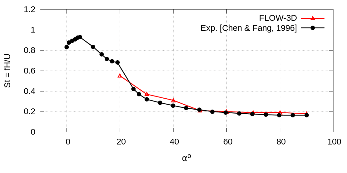
Figure 6: Vortex shedding in the wake of a beveled plate.
Each simulation was run for a total of $latex \displaystyle \bar{t}=\frac{t{{U}_{0}}}{H}=150$ dimensionless time units. For angles of inclination, α > 10° a regular pattern of vortex shedding can be seen in then the wake of the plate. This is illustrated qualitatively by a snapshot of TKE for the α=50° case in Figure 6b. The dominant frequency of vortex shedding in was estimated by counting the peaks in the time history of velocity magnitude at the same probe points used in the experiment. This was used to compute the associated Strouhal number, $latex \displaystyle St=\frac{fH}{{{U}_{0}}}$, which is plotted next to the experimental data in Figure 6c. Good agreement with the measured Strouhal number is achieved for all simulations where vortex shedding was predicted. For α= 0° and 10° the simulated flow behind the streamlined body did not exhibit a regular vortex shedding pattern. In these cases, a Large Eddy Simulation approach may be more capable of predicting the unsteady nature of the flow.
Bibliography
Berger, M., & Aftosmis, M. (2012). Progress towards a Cartesian cut-cell method for viscous compressible flow. 50th AIAA Aerospace Sciences Meeting Including the New Horizons Forum and Aerospace Exposition, (p. 1301).
Economon, T. D., Palacios, F., Copeland, S. R., Lukaczyk, T. W., & Alonso, J. J. (2016). SU2: An open-source suite for multiphysics simulation and design. AIAA Journal, 54, 828–846.
Gautier, R., Biau, D., & Lamballais, E. (2013). A reference solution of the flow over a circular cylinder at Re= 40. Computers & Fluids, 75, 103–111.
Gregory, N., & O’Reilly, C. L. (1970, 1). Low-speed aerodynamic characteristics of NACA 0012 aerofoil section, including the effects of upper-surface roughness simulating hoar frost. Tech. rep., NASA.
Grove, A. S., Shair, F. H., & Petersen, E. E. (1964). An experimental investigation of the steady separated flow past a circular cylinder. Journal of Fluid Mechanics, 19, 60–80.
Kirkpatrick, M. P., Armfield, S. W., & Kent, J. H. (2003). A representation of curved boundaries for the solution of the Navier–Stokes equations on a staggered three-dimensional Cartesian grid. Journal of Computational Physics, 184, 1–36.
Liang, Z. (2018, 10). Immersed Boundary Method for FLOW-3D. Technical Note, Flow Science, Inc.
Swamee, P. K., & Jain, A. K. (1976). Explicit equations for pipe-flow problems. Journal of the hydraulics division, 102, 657–664.
Tseng, Y.-H., & Ferziger, J. H. (2003). A ghost-cell immersed boundary method for flow in complex geometry. Journal of computational physics, 192, 593–623.
