

Turbulence
FLOW-3D offers a comprehensive turbulence modeling suite for fully 3-D flows, 2-D depth-averaged (shallow water) flows, and hybrid 3-D/2-D depth-averaged flows.There are eight available turbulence options in FLOW-3D.
The Prandtl mixing length model is one of the earliest attempts to describe three-dimensional turbulence effects. It is the least complex model, and is no longer widely used. FLOW-3D includes it mainly for its usefulness in academic studies.
The one-equation model is also an early effort to represent turbulence. It calculates time-averaged turbulent kinetic energy k and requires a known turbulent mixing length LT at all locations. Since LT is not usually known ahead of time, the one-equation model is not suitable for modeling complex flows.
The standard k-ε model (Harlow & Nakayama 1967) is a two-equation model that calculates both turbulent kinetic energy, k and dissipation rate, ε, and finds the turbulent mixing length LT dynamically. It is an industry standard, and has been found useful for representing a wide range of flows (Rodi 1980).
The Renormalized Group (RNG) k-ε model (Yakhot & Orszag 1986, Yakhot & Smith 1992) is a more robust version of the two-equation k-ε model, and is recommended for most industrial problems. It extends the capabilities of the standard k-ε model to provide better coverage of transitionally-turbulent flows, curving flows, wall heat transfer, and mass transfer.
The k-ω two-equation model (Wilcox 1988, 1998, 2008) defines the second variable not as turbulent dissipation ε but as ω ≡ ε/k (Kolmogorov 1942). Wilcox has improved upon the k-ω two-equation model since 1988 and in 1998 he introduced new coefficients that significantly improved the accuracy of the model for free shear flows. The k-ω two-equation model in FLOW-3D is thus suitable for modeling free shear flows with streamwise pressure gradients like spreading jets, wakes, and plumes.
The LES model does not use scalars to represent average turbulent kinetic energy, but rather resolves most of the turbulent fluctuations directly. It requires much finer mesh resolution than the two-equation models and provides more extensive statistics of the turbulent flow.
The 2-D depth-averaged shallow water turbulence model assumes a logarithmic fully-turbulent velocity. The first option assumes a constant drag coefficient CD, which may be spatially varied.
The second 2-D depth-averaged shallow water turbulence model makes the drag coefficient CD a dynamic function of fluid depth and spatially variable surface roughness.
Turbulence Simulations – A Model Comparison
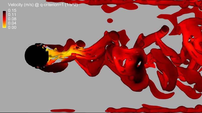
Fully 3-D tests indicate that time-averaging the LES model output gives results that are very similar to those of the two-equation Reynolds Averaged Navier-Stokes (RANS) models (standard k-ε, RNG k-ε, and k-ω), as shown in the fish passage videos below.
In the first video, a fish passage is simulated using FLOW-3D‘s large-eddy simulation (LES) turbulence model to analyze the magnitude of the velocity fluctuations. The second video shows time-averaged results from the same simulation. Here a simple customization shows that the time-average LES looks very similar to Reynolds-averaged Navier-Stokes (RANS) turbulence model results. The third video uses the same simulation to demonstrate using the Renormalized Group (RNG) k-ε turbulence model. The RNG k-ε model, like most Reynolds-averaged Navier-Stokes (RANS) turbulence models, treats the velocity fluctuations as isotropic scalar values and thus damps out the time-dependent velocity fluctuations. The results are similar to those found by time-averaging direct LES results, as shown in the second video.
References
- Driver, D.M. and Seegmiller, H.L., 1985, Features of a reattaching turbulent shear layer in divergent channel flow, AIAA Journal (23), 163-171.
- Harlow, F.H. and Nakayama, P.I., 1967, Turbulence transport equations, Physics of Fluids (10), 2323–2332.
- Harlow, F.H. and Nakayama, P.I., 1968, Transport of turbulence energy decay rate, Los Alamos Scientific Laboratory report LA-3854.
- Kolmogorov, A.N., 1942, Equations of turbulent motion in an incompressible fluid, Izvestia Academy of Sciences, USSR; Physics (6), 56-58.
- Pope, S. B, 2000, Turbulent Flows, Cambridge University Press.
- Rodi, W., 1980, Turbulence models and their application in hydraulics: a state of the art review, International Association for Hydraulic Research (IAHR), Delft, The Netherlands.
- Saffman, P.G., 1970, A Model for Inhomogeneous Turbulent Flow, Proceedings of the Royal Society London A (317), 417-433.
- Speziale, C.G, Abid, R., and Anderson, E.C, 1992, Critical evaluation of two-equation models for near-wall turbulence, AIAA Journal (30), 324-331.
- Wilcox, D. C., 1988, Reassessment of the scale-determining equation for advanced turbulence models, AIAA Journal (26), 1299-1310.
- Wilcox, D. C., 1998, Turbulence Modeling for CFD, DCW Industries, Inc., 2nd edition.
- Wilcox, D. C., 2008, Formulation of the k-omega turbulence model revisited, AIAA Journal (46), 2823-2838.
- Yakhot, V. and Orszag, S.A., 1986, Renormalization group analysis of turbulence I. Basic theory, Journal of Scientific Computing (1), 3-51.
- Yakhot, V. and Smith, L.M., 1992, The renormalization group, the e-expansion and derivation of turbulence models, Journal of Scientific Computing (7), 35-61.
