Numerical Treatment of Incompressible Flow
Table of Contents
The numerical treatment of fluid flow, now referred to as computational fluid dynamics (CFD), began in earnest during World War II. In the push to build an atomic bomb, considerable effort went into understanding the behavior and interactions of shock waves in a variety of materials. To aid in this effort, work was started on the building of digital computers that could carry out the huge number of arithmetic operations associated with numerical models of fluid dynamic processes. All CFD models were naturally designed for compressible fluids that exhibit shock waves. It was a number of years after the war, and when large computers became available for more general studies, that interest turned to methods for the numerical treatment of incompressible fluids.
Incompressible Flow Methods
The first (two dimensional) computational method for modeling incompressible fluids governed by the Navier-Stokes equations was published by Harlow and Welch in 1965 [1]. This method included a capability for general free surfaces existing in two-dimensional flows, another first. In addition, the Harlow and Welch paper introduced the concept of a staggered computational grid, something that is now a common practice (more about this later).
Those modeling compressible flows believed that their techniques, which considered fluids as continua satisfying a set of conservation equations and an equation of state, should be just as applicable to incompressible flows without any need for special treatment. They argued that it is only a matter of the speed of the fluid being less than the speed of sound in the fluid to be considered as incompressible. Actually, there are two conditions for a fluid to be considered incompressible. One is that the fluid speed must be less than the speed of sound in the fluid. A typical limit used in practice is that the fluid speed should be less than 0.3 times the speed of sound (i.e., a Mach number of 0.3). A second condition, rarely mentioned, is that the distance a sound wave travels in a characteristic time should be much larger than a characteristic length associated with the flow problem. This is illustrated in “The Incompressibility Assumption” article in this CFD-101 series).
To understand why compressible flow models are not suitable for incompressible flow, we will use a simple example of a one-dimensional channel of length L to illustrate the problem. Compressible fluid in the channel is at rest and has a gauge pressure of 0.0. The right end of the channel is closed and at the left end a piston pushes on the fluid causing a pressure p larger than the pressure in the channel to be imposed at time t=0. This causes a pressure pulse of magnitude p to travel from the left to the right, moving at the speed of sound c in the fluid. If the fluid is to be considered incompressible then it is expected that the fluid pressure would increase to equal the pressure applied by the piston so that it cannot move and change the volume of the fluid.
For this incompressible limit to happen, the compressible pressure waves in the fluid must traverse the length of the channel many times, reflecting back and forth between the ends of the channel until the pressures in the channel are smoothed to a uniform value sufficient to stop the piston. Users of compressible flow solvers require the simulation time-step size to remain small enough so that a pressure wave does not move more than one mesh cell width in one time step. So, to compute many wave transits across the channel requires a great many time steps. To limit the number of transits requires these users to introduce an averaging process of the pressures in each cell over some time interval. Unfortunately, this averaging still results in pressure fluctuations and does not produce the desired uniform pressure expected in an incompressible flow. Averaging more pressure wave transits would reduce the fluctuations, but the number necessary for a nearly uniform pressure would be much too large to be cost effective in terms of CPU usage.
The realization that compressible flow solvers cannot solve incompressible flows in an efficient way led to new developments designed explicitly for treating incompressible flow. The Harlow and Welch solution was to compute pressures that ensured a zero velocity divergence, which is the mathematical incompressibility condition. That is, the divergence of the velocity when integrated over a mesh cell (control volume) can be converted by Gauss’s theorem into the flux of volume crossing the boundary of the mesh cell. For incompressibility, this flux, which is the change in volume in the cell, must be zero.
Harlow and Welch devised an iterative solution to the divergence equal to zero equation when it is evaluated with the time advanced velocities,
(1) $latex \displaystyle \nabla \bullet \left( {{{\vec{u}}}^{n+1}} \right)=0$
They wrote approximations to the advanced velocity in the form,
(2) $latex \displaystyle {{\vec{u}}^{n+1}}=\tilde{u}-\frac{1}{\rho }\nabla {{p}^{n+1}}$
where ũ on the right side of the equation includes all the terms in the velocity equation (un, advection, viscous and body forces) except for the pressure gradient, which is to be evaluated at the advanced time. When Eq.2 is inserted into Eq.1 the result is a Poisson equation for the time advanced pressures. This equation must be solved iteratively. Originally, it was solved using a simple successive-over-relaxation (SOR) method. One difficulty with this approach is associated with boundary conditions. A pressure boundary is no problem (for example, at a free surface where the pressure is known), but a rigid wall that requires a zero normal velocity requires a special choice for the pressure in the wall that will ensure a zero normal velocity at the wall.
Convergence of the pressure iteration results in a velocity field that satisfies the incompressibility condition necessary for incompressible flows. Because Eq.1 is written in terms of the advanced time level n+1, the initial condition for this method does not have to satisfy a zero-divergence condition, since the flow after one time increment will be incompressible.
Reference [1] contains examples of flows computed using this model. However, to obtain these results, there is one more issue than needs to be addressed. When Harlow and Welch first tried to program Eq.1 they used a simple rectangular grid of mesh elements in which all variables (e.g., velocity components and pressures) were located at the centers of the elements, a common procedure at the time (see Plot 1).
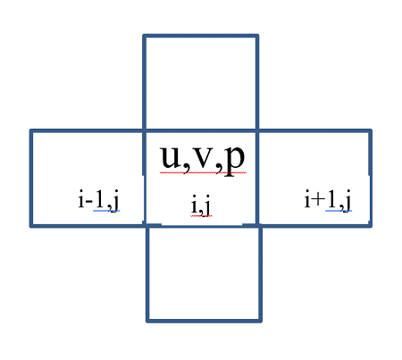
To write a difference equation for Eq.1 in the central grid element of Plot 1, the velocity at the right side of the cell would written as (ui,j+ui+1,j)/2 and at the left side (ui,j+ui-1,j)/2. The contribution to the divergence in Eq.1 would be the right-side velocity minus the left-side velocity divided by the width of the central element. As a result, Eq.1 for the central element does not involve the central element velocity u because it cancels out the difference of the velocities Likewise, the vertical velocity in the central element also does not appear in the divergence expression. A consequence of this is that the numerical solution generated using this grid layout decouples the velocities, much like a checkerboard where all the black squares are related, and all the red squares are related but the red and black squares are not coupled with one another.
To overcome this problem Harlow and Welch introduced a staggered grid arrangement, as shown in Plot 2. Here the u velocities are located at the centers of the left and right sides of the element, and the v velocities are located at the centers of the top and bottom of the element. The pressure remains in the center of the element.
With this arrangement, the pressure gradients on the edge velocities are evaluated over one cell width, while in the centered arrangement of Plot 1 the gradients are over 2 cell widths. This arrangement has a nice physical interpretation: if the velocities are fluxing out too much volume from the center cell, then reducing the center pressure will reduce the outflow at each edge of the cell; and if there is a net inflow of volume, an increase in the pressure will reduce the inflow at each edge.

In other words, a non-zero divergence can be changed to a zero divergence by simply changing the value of the central pressure. A difficulty with this is that if you change, for example, the u velocity on the right side of the cell, it will also change the divergence in the cell to the right. It is because of this problem that iterations are necessary to bring the divergences in all the cells to zero.
Wave Propagation
Pressure iterations can be crudely viewed in terms of wave propagation. Suppose a positive pressure is generated in a single mesh cell in the center of the one-dimensional channel previously described. This pulse will add to the pressures in its neighboring cells, each with half the value that is in the central cell. Those cells then transmit pulses to their neighbors again at half strength, now one fourth the original. Continuing further along the channel, the transmitted pulses get smaller and smaller. This is one crucial difference with the compressible flow pressure waves. Iterative pressure pulses exhibit a lot of damping, and when the amplitude of the pulses becomes less than the convergence level set for iterative pressure changes, the pulses are no longer propagated.
It is remarkable that in one paper Harlow and Welch introduced three major computational techniques for doing CFD. One of these is the staggered grid concept. The advantages of the staggered grid have made it a favorite scheme of many individuals involved in CFD.
An alternative method for computing incompressible flows was introduced in 1967 by A. Chorin, “A Numerical Method for Solving Incompressible Viscous Flow Problems,” [2]. Chorin introduced an artificial compressibility assumption using the equation,
(3) $latex \displaystyle \frac{\partial \rho }{\partial t}+\nabla \centerdot \vec{U}=0,$
$latex \displaystyle p=\frac{\rho }{\delta }$
Here p=ρ/δ is an artificial equation of state where δ is the artificial compressibility, analogous to a relaxation parameter. The effective sound speed is then c=1/δ1/2. This must be larger than any fluid speed in a computation to have an incompressible flow. An iterative computation would then consist of computing an estimate for the advanced velocities from the momentum equation to insert in Eq.3, which would give an updated density (and, therefore, pressure) to be used to adjust the advanced velocities to be consistent with the advanced pressures.
The advantage of Chorin’s scheme is that he used pressures and velocities directly, while Harlow and Welch only used pressures. This makes setting boundary conditions at solid walls much easier. Rather than having to establish a pressure on the inside of a solid wall, it is only necessary to set the normal velocity component to zero.
A disadvantage of Chorin’s scheme is the appearance of the δ parameter. He had no way to specify the value of δ and recommended one or more initial computations to determine a value that worked and that did not lead to instability.
Chorin did describe a simple observation inherent in the above scheme for incompressibility which is most easily understood in terms of the staggered grid arrangement shown in Plot 2. If the edge velocities of a mesh cell indicate a net outflow of volume from the cell, then lowering the pressure in the cell will reduce the outflow and conversely a net inflow can be eliminated by increasing the cell pressure.
With this simple interpretation connecting the pressure with the divergence it is a short step to realize how the Chorin and Harlow and Welch ideas can be combined for an even better method. Harlow and Welch’s technique of inserting the temporary velocities in the divergence shows how the pressures in the cell and in neighboring cells affect the divergence. Using only the coefficient of the cell pressure itself indicates how much it should be changed to drive the divergence toward zero. The reciprocal of this coefficient is the optimum choice for Chorin’s parameter δ. More importantly, this parameter will not be a constant, as it is in Chorin’s method, because it will automatically take into account fixed velocities at boundary walls. This variation increases the convergence rate of the iteration scheme.
In summary, the most frequently used technique for computing incompressible flows uses temporary estimates for the time-advanced velocities that are then used to compute a divergence. A change in cell pressure is computed from this divergence that in turn drives the divergence in the cell to zero. The change in pressure that does this is added to the velocity components in the cell. Repeating this in every mesh cell and then repeating it over the entire mesh eventually leads to convergence. It is usually recommended that an over-relaxation parameter be introduced to increase the pressure changes in a cell to compensate for the fact that this change will be reduced by competing changes in neighboring cells. Of course, there are many iterative methods than can be used to achieve the necessary coupling between pressures and velocities that will result in a zero-velocity divergence. They all, however, boil down to a variant of what has been presented here.
References
- H. Harlow and, J.E. Welch, “Numerical Calculation of Time-Dependents Viscous Incompressible Flow of Fluid with Free Surface,” Phys. Fluids 8, 2182 (1965).
- J. Chorin, “A Numerical Method for Solving Incompressible Viscous Flow Problems,” J. Comp. Physics, 2, 12 (1967)