


What's New in FLOW-3D HYDRO 2025R1
FLOW-3D HYDRO 2025R1 introduces a new discrete element method (DEM) model. This model allows users to account for particle-particle interactions such as collision and friction, providing utility beyond that of the standard Lagrangian particle model.
Various scenarios in water and environmental projects involve rocks or riprap. Some examples include natural channel beds or as part of channel and structure protection systems. The DEM model can provide insights into rock stability under different flow conditions, opening exciting possibilities for cost savings and risk reduction for unique protection systems on riverbanks and other structures.

This model can also help users gain insights into grit separation systems, stormwater separators, and other scenarios where small objects interact with each other.

Note: This model requires a separate license token, which can be added at an additional cost. Please contact sales@flow3d.com to request access.
What's New in FLOW-3D HYDRO 2024R1

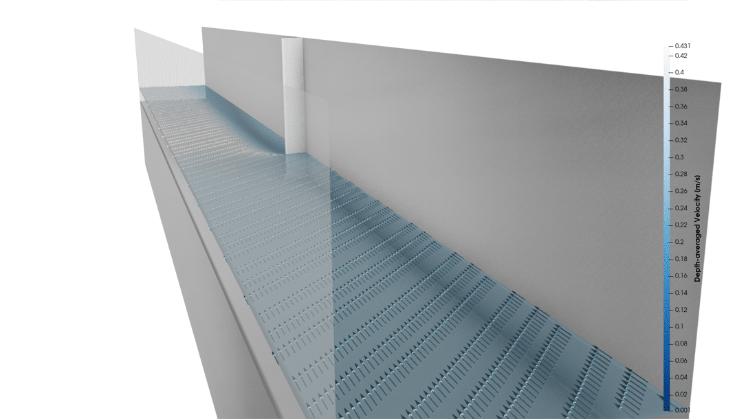
A second development for FLOW-3D HYDRO is to include LandXML and the triangulated raster surfaces into the EXODUS II-based output files. This makes the full topography/bathymetry available when postprocessing, making it easier to convey results to your audience in a way that focuses on the story rather than the modeling details.

What's New in FLOW-3D HYDRO 2023R2
New results file format
We introduced an all-new results file format based on the EXODUS II format, enabling faster postprocessing in FLOW-3D HYDRO and FLOW-3D POST 2023R2. This new file format significantly reduces the time spent on postprocessing tasks for large, complex simulations (up to 5x on average!) while improving connectivity with other visualization tools.
Users now have the choice to write Selected data in either flsgrf, EXODUS II, or both flsgrf and EXODUS II file formats. The new EXODUS II file format utilizes finite element meshes for each object, which allows users to also open FLOW-3D HYDRO results with other compatible postprocessors and FEA codes. With the new workflow, users can visualize large, complex cases quickly and extract auxiliary information using arbitrary slicing, volume renders, and statistics.

The new results file format boasts a remarkable speed-up in visualization workflows compared to flsgrf without sacrificing the performance of the hydr3d solver. This exciting new development provides a seamless simulation experience with improved speed and flexibility in results analysis.
Learn more about the new visualization capabilities in FLOW-3D POST.
Turbulence model improvements
FLOW-3D HYDRO 2023R2 brings a major improvement to the dynamic mixing length calculation for two-equation (RANS) turbulence models. In certain limiting cases such as near-laminar flow regimes, the code-computed limiter could in previous versions sometimes be overpredicted, forcing the user to manually input a specific mixing length.
The new dynamic mixing length calculation better accounts for the turbulent length and time scales in these situations, and users can now apply the dynamic model to a wider range of flows instead of setting a fixed (physics-based) mixing length.

Hydrostatic pressure initialization
It is often necessary for users to initialize hydrostatic pressure in pre-defined fluid regions. Previously in large, complex simulations, the hydrostatic pressure solver could sometimes be slow to converge. FLOW-3D HYDRO 2023R2 brings a significant performance improvement to the hydrostatic solver, enabling it to converge up to ~6x faster during the preprocessing stage.
Expanded terrain representation support
GeoTIFF support
With the 2023R2 release, FLOW-3D HYDRO natively supports the GeoTIFF (.tif) file format for raster topography and bathymetry. Users can now directly import GeoTIFF files into the user interface.

LandXML support
In cases where survey data is non-uniform or raster surfaces do not have sufficient resolution, TIN surfaces offer an improved map of the topography via the LandXML (.xml) file format. FLOW-3D HYDRO 2023R2 natively imports LandXML files.
Improved interactivity with raster files
Raster files often cover large topographic areas at high resolution, which can slow down the interactivity of the 3D representation in the user interface. Users can now control the quality of the 3D representation, greatly reducing the rendering time and significantly improving interactivity.
What's New in FLOW-3D HYDRO 2023R1
Shallow water turbulence models
Turbulence is a key aspect of water and environmental flow fields, especially so in regimes modeled with shallow water approximations. We enhanced our treatment of turbulence in our shallow water model to include three new turbulence models, the constant diffusivity, mixing length, and Smagorinsky models, to help reduce modeling risk and give better results.
What's New in FLOW-3D HYDRO 2022R2
With the release of FLOW-3D HYDRO 2022R2, Flow Science has unified the workstation and HPC versions of FLOW-3D HYDRO to deliver a single solver engine capable of taking advantage of any type of hardware architecture, from single node CPU configurations to multi-node parallel high performance computing executions. Additional developments include improved entrained air functionalities, as well as boundary condition definition improvements for water and environmental applications.
Unified solver
We migrated our FLOW-3D products to a single, unified solver to run seamlessly on local workstations or on high performance computing hardware environments.
Many users run their models on laptops or local workstations, but in addition run larger models on high performance computing clusters. With the 2022R2 release, the unified solver allows users to exploit the same benefits of OpenMP/MPI hybrid parallelization from HPC solutions to run on workstations and laptops.


Multi socket workstations
Multi socket workstations are now very common and capable of running large simulations. With the new unified solver, users using this type of hardware will generally see performance gains from being able to run models taking advantage of OpenMP/MPI hybrid parallelization that used to be only available on HPC cluster configurations.
Low level routines improved vectorization and memory access
Performance gains on the order of 10% to 20% have been observed for most test cases, with some cases yielding run-time benefits in excess of 20%.
Refined volumetric convective stability limit
Time step stability limit is a major driver in model runtime, with 2022R2, a new time step stability limit, 3D convective stability limit, is available in the numerics widget. For models that are running and convection limited (cx, cy, or cz limits) the new option has shown typical speed-ups on the order of 30%.
Pressure solver pre-conditioner
In some cases, for challenging flow configurations, run times can be drawn out due to excessive pressure solver iterations. For those difficult cases, with 2022R2, when a model iterates too heavily, FLOW-3D automatically activates a new pre-conditioner to help with pressure convergence. Tests have improvements in runtime anywhere from 1.9 to 335 faster!
Log conformation tensor method for visco-elastic fluids
A new solver option for visco-elastic fluids is available to our users, and is particularly effective for high Weissenberg numbers.
FLOW-3D HYDRO boundary conditions refinements
Two improvements for water application boundary conditions are available in FLOW-3D HYDRO 2022R2. Shallow water volume flow rate boundary conditions have been improved to yield more realistic, spatially-varying velocity profiles so users can reduce the domain size without losing accuracy. For natural inlet boundary conditions, the response to transient conditions can be improved with the use of the rating curve relaxation time option.

Improved entrained air functionalities
For diffusers and similar bubble flow applications, mass sources can now be used to introduce air into the water column. In addition, default values for the turbulent diffusion of entrained air and dissolved oxygen have been updated.

What's New in FLOW-3D HYDRO 2022R1
The new 2022R1 versioning of FLOW-3D products reflects Flow Science’s adoption of a synchronized release naming convention for FLOW-3D, FLOW-3D CAST and FLOW-3D HYDRO. 2022R1 represents the transition to a unified code base for FLOW-3D products. This important evolution will allow users access the latest developments as soon as they are ready, at a more frequent product release pace.
The FLOW-3D HYDRO 2022R1 release features an extension to the FAVOR™ method called detailed cutcell representation, new dissolved oxygen and axial pump models, extensions to Active Simulation Control capabilities, tabular properties which allow users to specify complex property dependencies based on two independent variables, and additional numerics features such as a VOF-to-particle development to improve mass conservation for fluid regions subject to breakup.
Detailed Cutcell Representation – An Extension to FAVOR™
The FAVOR™ method represents solid geometry using area and volume fractions on a regular, Cartesian grid. It enables FLOW-3D HYDRO to efficiently simulate flow through and around complex geometry without resorting to unstructured body-fitted meshes. One challenge for the FAVOR™ method is computing accurate wall shear stresses along solid surfaces that do not align with a mesh plane. An extension to FAVOR™ called detailed cutcell representation greatly improves the calculation of wall shear stresses, resulting in significant improvements in the calculation of drag forces on solid surfaces as well as pressure drops along surfaces and in channels.
Learn more about the advanced numerics as well as validations of the detailed cutcell representation.

Dissolved Oxygen Model
Dissolved oxygen in water plays an important role in natural and manmade habitats. Acceptable levels of dissolved oxygen is a key indicator of water quality. In wastewater treatment plants, oxygen feeds bacteria that break down contaminants. FLOW-3D HYDRO‘s new dissolved oxygen model is coupled with the air entrainment, drift-flux and dynamic bubble size models, creating a consistent approach to modeling air bubble and dissolution dynamics. The mass transfer coefficient between the bubbles and water can be specified in one of three ways: as a user-defined constant, through a “clean” bubble assumption using Higbie’s model, or through a “dirty” bubble assumption which accounts for the effects of surfactants on oxygen dissolution.
In this simulation, oxygen bubbles are injected from two diffusers at the bottom of the container and allowed to rise in water. As the bubbles rise, oxygen dissolves into water. The image on the left shows the concentration of dissolved oxygen in water. The image on the right shows the water velocity which is induced by the rising oxygen bubbles.
Expanded Controls for Active Simulation Control
Active Simulation Control (ASC) is very useful for controlling simulations based on flow information at probes. In this release, ASC has been expanded to allow additional controls based on flow information from general history data, flux surfaces, and sampling volumes.
One of the advantages of flux surfaces and sampling volumes over point probes is that they can provide information that is averaged over a surface or a volume rather than point-based. In some situations, surface-based and volume-based information can be more representative of the behavior of interest in simulations.
With this new capability, users can:
- Terminate a simulation when the temperature in a control volume exceeds or falls below a critical value.
- Open and close valves when the mass or volume of fluid in a control volume reaches the specified values.
- Control the filling rate from a nozzle based on the turbulent energy in a sampling volume.
- Control the output frequency based the average velocity on flux planes.
- Terminate a simulation when fill fraction in a sampling volume reaches the value specified by the user.
This example represents a sludge decanter that models a mixture of water and sludge entering a decanter and separating. Water is allowed to flow in and out at the back side of the decanter to maintain a relatively fixed level in the decanter. A sampling volume in the bottom of the decanter is used to measure the amount of sludge captured at the bottom. When the sludge mass in the sampling volume reaches 200 kg, a valve opens to release the sludge. The valve closes when the sludge mass drops below 180 kg.
Axial Pump Model
FLOW-3D HYDRO’s new axial pump model allows users to mimic the net effect of an axial pump in their simulations. There are two options with respect to the pump behavior. The first option is to prescribe either a volumetric flow rate or a flow velocity through the pump so that the fluid is moved at the specified rate. This option is appropriate when an operating flow rate is provided for the pump. The second option provides a more complete definition of the pump operation based on a pump performance curve. In this case, the user can define a linear approximation of the pump’s performance curve so that the flow rate through the pump will depend on the pressure drop across the pump. In this configuration, the typical behavior of a pump is represented, whereby the flow will slow down and eventually stall as a reverse dynamic head builds up and pushes back against the pump operation.
In the GUI, users can define component-based pumps using a dynamic view based on Fan/Impeller or Axial pump components, where the flow rate is prescribed using a momentum source.


Tabular Properties
Material properties such as viscosity and surface tension can be dependent on flow conditions such as temperature, density, strain rate, or user-defined scalar quantities representing things like a contaminant concentration. Fitting these properties to functional forms can require complex curve-fitting, especially when the properties are dependent on more than one independent variable. The new tabular properties feature in FLOW-3D HYDRO allows users to define fluid properties in table form with up to two independent variables. For example, surface tension can be tabulated from experimental data to describe complex, non-linear dependencies on contaminant concentration and temperature, or viscosity can be tabulated from experimental data to represent a dependency on strain rate and temperature. Users can input a single variable or two variable dependency in the tabular properties dialog.
Viscosity is defined as a function of both solid content (density) and strain rate. In this example a dense fluid region slides down into a quiescent pool which at time zero is layered with a dense settled fluid region and clear water above.
VOF to Particles
The accuracy and robustness of the sharp-interface tracking VOF methods in FLOW-3D HYDRO have been enhanced by combining them with fluid particles. The new particle species, called VOF particles, are used in place of the VOF function to track small fluid ligaments and droplets in the computational domain, achieving better conservation of fluid volume and momentum.
Higher time steps size can also be expected in gravity-controlled processes. The VOF fluid is automatically converted to VOF particles at certain times and locations when certain conditions are met. The particle motion is then calculated using the Lagrangian particle model and the particles are converted back to the VOF representation upon reentering the fluid.
Time-dependent Valves
Valves may be used in water transport simulations where it is vital to maintain adequate pressures to support structural stability. Valves can now be controlled based on time. This feature is useful for representing valves that are activated at specified times in a defined control sequence to determine system operating characteristics.


What's New in FLOW-3D HYDRO v1.0
FLOW-3D HYDRO’s new streamlined user interface focuses on the needs of the water community. A ‘What You See Is What You Need’ (WYSIWYN) approach to model setup, application-specific workspace templates, and a new library of simulation examples promote unparalleled workflow efficiency, while access to high performance computing options and continued development of advanced solver capabilities deliver a state-of-the-art CFD modeling solution for water infrastructure & environmental engineering applications. FLOW-3D HYDRO continues to uphold Flow Science’s core commitment to first class technical support and customer service.
Streamlined GUI for W&E Practitioners
FLOW-3D HYDRO’s streamlined user interface features workflows designed for civil & environmental applications, providing effective, accurate and error-free modeling.
User success is achieved through:
- Immediate access to relevant modeling features and parameter selection options
- Removal of unnecessary information, allowing for superior modeling clarity and modeling outcomes
- A faster, more sequential workflow with enhanced visibility of important settings, meaning fewer places to make mistakes
- Convenient defaults that save you time and remove repetitive entries
- Help and guidance when you need it
- A new extended examples library covers a wide range of model problems from simple to complex example use cases
- Video tutorials and templates provide additional immediate guidance for the most challenging modeling needs
Simulation Templates
Save time, avoid mistakes, and run consistent models with FLOW-3D HYDRO’s Workspace Templates. Workspace Templates pre-load fluid properties, physical models, numerical settings and simulation outputs for common applications.
Workspace Templates are available for seven classes of models:
- Free surface – TruVOF (default)
- Air entrainment
- Thermal plumes
- Sediment transport
- Shallow water
- Free surface – 2 fluid VOF
- No free surface
Pre-loaded Example Simulations
FLOW-3D HYDRO’s library of over forty pre-loaded water-focused example simulations provide a great starting point for modeling your application. Pre-loaded example simulations give modelers a detailed starting point for most applications as well as a roadmap of model setups and best practices.
Video Tutorials
Video tutorials provide an excellent route for new users to quickly learn how to model a wide variety of applications. FLOW-3D HYDRO video tutorials feature:
- A-Z step-by-step recording for a wide range of application and physics
- “How-to” information
- Tips for best practices
- CAD/GIS data, simulation files and post-processing files
Advanced Solver Developments
Tailings Model
The new tailings model provides advanced capabilities for simulating tailings runout due to tailings dam failure. A bi-modal viscosity model representing fine and coarse particle compositions along with a multi-layer approach to tailings definition allows for modeling of tailings dams constructed by any method. Flexible meshing, including shallow water, 3D, and hybrid 3D/shallow water meshing allows the complexity of multi-layered tailings to be accurately modeled while providing fast solutions in shallow regions. A two-layer Herschel-Bulkley viscosity model is available for shallow water meshes for accurate representation of viscous boundary layers.
Model Highlights
- Bi-modal viscosity model for fine and coarse particle tailings compositions
- Tailings transport including settling, packing, and turbulent diffusion of particle species
- Two-layer Herschel-Bulkley viscosity model for shallow water meshes
- Flexible meshing approaches including 3D, shallow water, and 3D/shallow water hybrid meshes
- Multi-layer, variable composition tailings for general definition of tailings dam construction
Shallow Water
FLOW-3D HYDRO’s shallow water modeling capabilities employ unique hybrid meshing that allow 3D meshes to be combined with shallow water meshes for exceptional modeling versatility. Numerical improvements to the pressure solver have resulted in more stable, faster simulations. The bottom shear stress calculations in hybrid meshes have been greatly improved, further increasing their accuracy. New methods of applying roughness to topography include Strickler, Chezy, Nikuradse, Colebrook-White, Haaland, and Ramette equations.
Two-Fluid VOF Model
A two-fluid model, with or without a sharp interface, compressible or incompressible, has always been available in FLOW-3D along with the one-fluid free-surface model. In fact, the sharp interface treatment shares the TruVOF technology with the free surface model and is unique in commercial CFD software. Recent developments included two-field temperature and interface slip models. The model has been successfully applied to oil/water, liquid/vapor, water/air and other two-phase systems.
FLOW-3D HYDRO sees two important advances in the accuracy and stability of the two-fluid solution. An enhanced coupling of the momentum and mass conservation equations improves momentum conservation at the interface, especially for liquid/gas flows. Expanded approximations of the limited compressibility terms in the continuity equation result in a faster and more stable two-fluid pressure solver.
Both developments are timely for the FLOW-3D HYDRO release, as air often plays a crucial role in hydraulic applications, for example, in tunnels and dropshaft designs. Limited compressibility is typically used for water and air in such cases due to typically low Mach numbers.
High Performance Computing and the CLOUD

While much work can be done with regular workstations or even laptops, large simulations as well as high definition simulations benefit immensely from tapping into more CPU cores. FLOW-3D CLOUD and High Performance Computing deliver just that: faster runtimes and more choices to run larger, more accurate models. To learn more about how FLOW-3D HYDRO can be installed on your in-house HPC cluster, flexible options for deploying on FLOW-3D CLOUD or our HPC Services, please contact us. The net result? A simulation that might take four to five days to run on an 8 core workstation will often be completed overnight on a 160 cores HPC solution, whether in-house on your local cluster, or running on as few as four nodes on FLOW-3D CLOUD.