FLOW-3D v12.0 marks an important milestone in the design and functionality of the graphical user interface (GUI), which simplifies model setup and improves user workflows. A state-of-the-art Immersed Boundary Method brings greater accuracy to FLOW-3D v12.0’s solution. Other featured developments include the Sludge Settling Model, the 2-Fluid 2-Temperature Model, and the Steady State Accelerator, which allows users to model their free surface flows even faster.
Physical & Numerical Models
Accurate prediction of forces and energy losses is crucial to the success of modeling many engineering problems involving flows around solid bodies. The release of FLOW-3D v12.0 features a new ghost-cell based Immersed Boundary Method (IBM) designed for such problems. IBM provides a more accurate solution near walls for internal and external flows, improving the calculation of drag and lift forces.
The two-fluid heat transfer model has been extended to separate energy transport equations for each fluid. Each fluid now has its own temperature variables, which improves the accuracy of the heat and mass transfer solutions near the interface. Heat transfer at the interface is now controlled by a user-defined heat transfer coefficient that can be a tabular function of time.
The new sludge settling model, a valuable addition for municipal applications, allows users to model the solid waste dynamics in water treatment tanks and clarifiers. Unlike the drift-flux model, where the settling velocity is a function of the droplet size of the dispersed phase, the settling velocity is a function of sludge concentration and can be input in both functional and tabular form.
As the name implies, the steady-state accelerator quickens the approach to a steady state solution. This is achieved by damping small-amplitude gravity and capillary surface waves, and is applicable only to free surface flows.
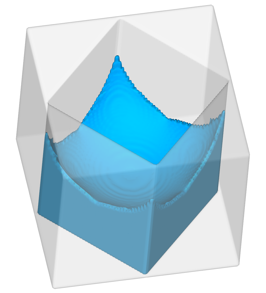
Void particles have been added to the bubble and phase change model. Void particles represent collapsed void regions, acting as small bubbles that interact with the fluid via drag and pressure forces. Their size changes in response to the surrounding fluid pressure, and their final location at the end of the simulation indicates a potential for air entrainment.
The sediment transport and erosion model has been overhauled to enhance its accuracy and stability. In particular, the mass conservation for sediment species has been greatly improved.
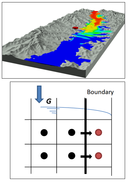
The fixed-pressure boundary condition now includes an ‘outflow’ option, where all flow quantities except for pressure and fluid fraction reflect the flow conditions upstream of that boundary. The outflow pressure boundary condition is a hybrid of a fixed-pressure and continuity boundary conditions.
Particle sources can now move during a simulation. Time-dependent translational and rotational velocities are defined in a tabular form. The motion of a particle source is added to the initial velocity of the particles emitted at the source.
In the gravity and non-inertial reference frame model, the location of the center of gravity as a function of time can be defined as a table in an external file. This feature is useful when modeling, for example, a rocket that is expending fuel and separating stages.
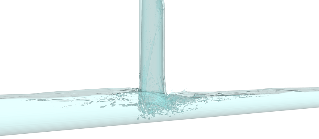
The simplest volume-based air entrainment model option has been replaced by the existing mass-based model. The mass-based model is more physics-based since, unlike volume, entrained air mass is conserved while its volume changes in response to the surrounding fluid pressure.
Tracers generated at flux surfaces can now diffuse due to molecular and turbulent diffusion processes, mimicking the behavior of real pollutants, for example.
Model Setup
The units system must now be fully defined, including temperature. Standard unit systems are provided. Additionally, the user can define units for mass, time and length from a selection of options, allowing for customized and convenient units. The user must also specify whether pressures are defined in gauge or absolute units. Default simulation units can be set in Preferences. The full definition of the units allows FLOW-3D to define default values for physical quantities as well as set universal constants, thus minimizing the amount of work required by the user.
Manning’s roughness in shallow water model
The Manning’s roughness coefficient has been implemented in the shallow water model for the evaluation of the shear stress at the terrain surface. It complements the existing roughness model based on the size of surface imperfections, and can be used in combination with it. As with the standard roughness, the Manning’s coefficient can be an attribute of a component or subcomponent, or can be imported from a terrain raster data set.
Mesh generation
Mesh setup for the vertical direction has been simplified by requiring only the definition of the bottom and top boundary coordinates.
Users can now apply rotational, translational and scaling transformations to components consisting of multiple subcomponents, simplifying the process of setting up complex geometry assemblies. For a General Moving Object (GMO) component, these transformations can be applied to the body-fitted coordinate system so that it is aligned with the component’s symmetry axes.
Active Simulation Control has been extended to heat sources associated with geometry components. The release of heat can now be controlled by history probes.
Fluid temperature at mass and mass/momentum sources can now be defined as a function of time using tabular input.
Emissivity coefficients for radiative heat transfer to voids are now defined directly, instead of requiring the user to specify the product of emissivity and the Stefan-Boltzmann constant. The latter is now automatically set by the solver, based on the units system.
- Flow velocities can now be output to Selected data when using the constant velocity field solver option.
- Torque on geometry components due to wall adhesion is output to General History data as a separate quantity, in addition to the existing output of wall adhesion forces.
- Shear velocity and y+ are automatically output to Selected data along with turbulent energy and dissipation, when turbulence model output is requested.
- Several quantities have been added to the air entrainment model output. The volume flux of entrained air and of escaping air in every cell containing free surface is output to Restart and Selected data, providing the user with detailed information of where and when air is being entrained and detrained. The time- and space-integrated equivalents of those two quantities in the whole computational domain, as well as for each Sampling Volume, are output to the General History
- The final size of the solver’s output file, flsgrf, is reported at the end of the simulation.
- For two-fluid simulations, the existing output quantities fluid residence time and distance traveled by fluid are now computed separately for fluid #1 and #2 and for the mixture of the fluids.
- For mass particles, the total volume and mass of each species are computed and output to General history for the whole computational domain, Sampling Volumes and Flux Surfaces, complementing the current output for the particle species counts.
- The last local gas pressure has been added as an optional output quantity to help the user identify gas entrapment and to assist in designing the venting system in fuel tanks, for example. That quantity records the last void pressure in a cell before it is filled with fluid and is used in combination with the adiabatic bubble model.
In the gravity and non-inertial reference frame model, the location of the center of gravity as a function of time can be defined as a table in an external file. This feature is useful when modeling, for example, a rocket that is expending fuel and separating stages.
New user-customizable source routines have been added and can be accessed in the user’s development environment:
Source routine name | Description |
cav_prod_cal | Cavitation production and dissipation rates |
sldg_uset | Sludge settling velocity |
phchg_mass_flux | Mass flux due to evaporation and condensation |
flhtccl | Heat transfer coefficient between fluid #1 and #2 |
dsize_cal | Coalescence and breakup rates for the dynamic droplet size model in two-phase flows |
elstc_custom | Source terms in the stress equations for viscoelastic fluids |
Brand New User Interface
Setup dock widgets
All setup operations, including Physics, Fluids, Mesh, and FAVOR™, have been converted into dock widgets around the geometry window, allowing Model Setup to be condensed into a single tab. With this transition, the crowded collapsible trees from prior versions have been replaced with a much cleaner, more efficient menu presentation, providing users easy access to every parameter without ever leaving the Model Setup tab.
New Model Setup icons
With our new Model Setup design comes new icons, representing each step of the setup process.
New Physics icons
Our Physics icons are designed to be easily differentiated from one another at a glance, while providing clear visual representation of each model’s purpose and use.
RSS feed
The Simulation Manager tab has been revamped for FLOW-3D v12.0, starting with the new RSS Feed. Upon launching FLOW-3D, users are now greeted with the latest news, events, and blog posts from Flow Science.
Configurable simulation monitor
An important task when running simulations is monitoring them. In FLOW-3D v12.0, the Simulation Manager has increased plotting capabilities to help the user better monitor their simulations. The user can select from all available general history data variables to monitor via the simulation runtime graphs and can add multiple variables to each graph. General history data available at runtime now includes:
- Minimum/maximum fluid temperatures
- Temperatures at probe locations
- Flow rates at flux surface locations
- Simulation diagnostics (e.g., time step, stability limits)
Conforming mesh visualization
Users can now visualize conforming mesh blocks via the new FAVOR™ dock widget.
Large raster and STL data
Processing large geometry data can be painstaking, due to the amount of time it takes for the data to be processed. While processing large geometry data can still take a significant amount of time, FLOW-3D now loads these large data sets as background tasks, allowing the user to continue working in a fully responsive, uninterrupted interface while their data is being processed.